Running Classic Monte Carlo
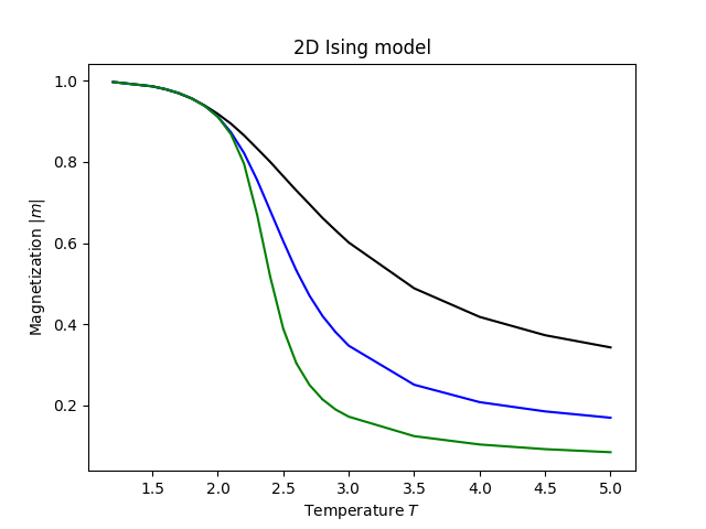
As a simple example for classic Monte Carlo we consider obtaining a phase transition in 2D Ising model.
First step we need to import required packages
import pyalps
import matplotlib.pyplot as plt
import pyalps.plot
Prepare the input parameters
parms = []
for l in [4,8,16]:
    for t in [5.0,4.5,4.0,3.5,3.0,2.9,2.8,2.7]:
        parms.append(
            {
              'LATTICE'        : "square lattice",
              'T'              : t,
              'J'              : 1 ,
              'THERMALIZATION' : 1000,
              'SWEEPS'         : 400000,
              'UPDATE'         : "cluster",
              'MODEL'          : "Ising",
              'L'              : l
            }
    )
    for t in [2.6, 2.5, 2.4, 2.3, 2.2, 2.1, 2.0, 1.9, 1.8, 1.7, 1.6, 1.5, 1.2]:
        parms.append(
            {
              'LATTICE'        : "square lattice",
              'T'              : t,
              'J'              : 1,
              'THERMALIZATION' : 1000,
              'SWEEPS'         : 40000,
              'UPDATE'         : "cluster",
              'MODEL'          : "Ising",
              'L'              : l
            }
    )
Here we consider lattices of sizes $4\times 4$, $8\times 8$, $16\times 16$, for different temperatures.
After that we write the input into ALPS specific format and run spin Monte Carlo simulation (spinmc):
#write the input file and run the simulation
input_file = pyalps.writeInputFiles('parm7a',parms)
pyalps.runApplication('spinmc',input_file,Tmin=5)
After the simulation is finished we can evaluate and plot the results.
pyalps.evaluateSpinMC(pyalps.getResultFiles(prefix='parm7a'))

#load the susceptibility and collect it as function of temperature T
data = pyalps.loadMeasurements(pyalps.getResultFiles(prefix='parm7a'),['|Magnetization|'])
magnetization_abs = pyalps.collectXY(data,x='T',y='|Magnetization|',foreach=['L'])

#make plots
plt.figure()
pyalps.plot.plot(magnetization_abs)
plt.xlabel('Temperature $T$')
plt.ylabel('Magnetization $|m|$')
plt.title('2D Ising model')
plt.show()
After that we should obtain the following figure for magnetization in 2D Ising model
