Running QMC simulation
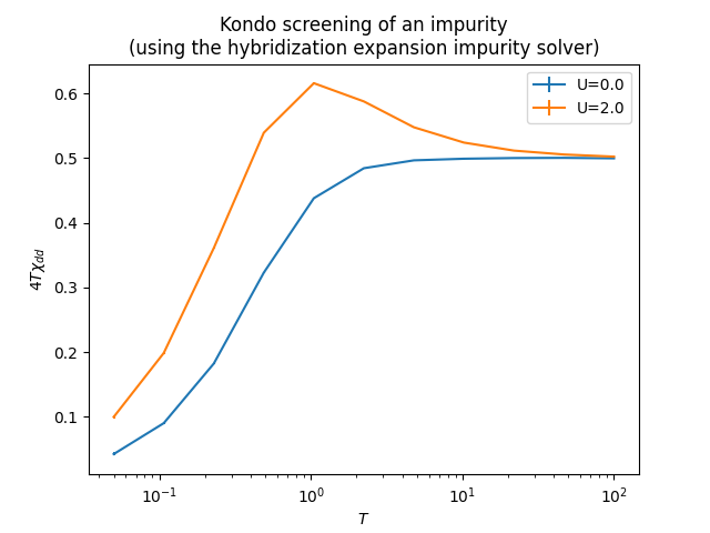
As an example for Quantum Monte Carlo simulation we show simulation of the effective local moment of the impurity with decreasing temperature due to Kondo screening, with semielliptical density of states is used as a hybridization function.
First we import all required python modules
from pyalps.hdf5 import archive       # hdf5 interface
import pyalps.cthyb as cthyb      # the solver module
import matplotlib.pyplot as plt   # for plotting results
from numpy import exp,log,sqrt,pi # some math
Generate a sequence of $10$ temperatures between $0.05$ and $100.0$ which are equidistant on a logarithmic scale
N_T  = 10    # number of temperatures
Tmin = 0.05  # maximum temperature
Tmax = 100.0 # minimum temperature
Tdiv = exp(log(Tmax/Tmin)/N_T)
T=Tmax
Tvalues=[]
for i in range(N_T+1):
  Tvalues.append(T)
  T/=Tdiv
Set up the values of onsite interaction, number of time points and timelimit for each simulation
Uvalues=[0.,2.] # the values of the on-site interaction
N_TAU = 1000    # number of tau-points; must be large enough for the lowest temperature (set to at least 5*BETA*U)
runtime = 5     # solver runtime (in seconds)
Setup the parameters for the simulation
values=[[] for u in Uvalues]
errors=[[] for u in Uvalues]
parameters=[]
for un,u in enumerate(Uvalues):
    for t in Tvalues:
        # prepare the input parameters; they can be used inside the script and are passed to the solver
        parameters.append(
         {
           # solver parameters
           'SWEEPS'             : 1000000000,                         # sweeps to be done
           'THERMALIZATION'     : 1000,                               # thermalization sweeps to be done
           'SEED'               : 42,                                 # random number seed
           'N_MEAS'             : 10,                                 # number of sweeps after which a measurement is done
           'N_ORBITALS'         : 2,                                  # number of 'orbitals', i.e. number of spin-orbital degrees of freedom or segments
           'BASENAME'           : "hyb.param_U%.1f_BETA%.3f"%(u,1/t), # base name of the h5 output file
           'MAX_TIME'           : runtime,                            # runtime of the solver per iteration
           'VERBOSE'            : 1,                                  # whether to output extra information
           'TEXT_OUTPUT'        : 0,                                  # whether to write results in human readable (text) format
           # file names
           'DELTA'              : "Delta_BETA%.3f.h5"%(1/t),          # file name of the hybridization function
           'DELTA_IN_HDF5'      : 1,                                  # whether to read the hybridization from an h5 archive
           # physical parameters
           'U'                  : u,                                  # Hubbard repulsion
           'MU'                 : u/2.,                               # chemical potential
           'BETA'               : 1/t,                                # inverse temperature
           # measurements
           'MEASURE_nnw'        : 1,                                  # measure the density-density correlation function (local susceptibility) on Matsubara frequencies
           'MEASURE_time'       : 0,                                  # turn of imaginary-time measurement
           # measurement parameters
           'N_HISTOGRAM_ORDERS' : 50,                                 # maximum order for the perturbation order histogram
           'N_TAU'              : N_TAU,                              # number of imaginary time points (tau_0=0, tau_N_TAU=BETA)
           'N_MATSUBARA'        : int(N_TAU/(2*pi)),                  # number of Matsubara frequencies
           'N_W'                : 1,                                  # number of bosonic Matsubara frequencies for the local susceptibility
           # additional parameters (used outside the solver only)
           't'                  : 1,                                  # hopping
           'Un'                 : un,                                 # interaction point
         }
        )
For each set of parameters setup hybridization function
for parms in parameters:
    ar=archive(parms['BASENAME']+'.out.h5','a')
    ar['/parameters']=parms
    del ar
    print("creating initial hybridization...").
    g=[]
    I=complex(0.,1.)
    mu=0.0
    for n in range(parms['N_MATSUBARA']):
        w=(2*n+1)*pi/parms['BETA']
        g.append(2.0/(I*w+mu+I*sqrt(4*parms['t']**2-(I*w+mu)**2))) # use GF with semielliptical DOS
    delta=[]
    for i in range(parms['N_TAU']+1):
        tau=i*parms['BETA']/parms['N_TAU']
        g0tau=0.0;
        for n in range(parms['N_MATSUBARA']):
            iw=complex(0.0,(2*n+1)*pi/parms['BETA'])
            g0tau+=((g[n]-1.0/iw)*exp(-iw*tau)).real # Fourier transform with tail subtracted
        g0tau *= 2.0/parms['BETA']
        g0tau += -1.0/2.0 # add back contribution of the tail
        delta.append(parms['t']**2*g0tau) # delta=t**2 g

    # write hybridization function to hdf5 archive (solver input)
    ar=archive(parms['DELTA'],'w')
    for m in range(parms['N_ORBITALS']):
        ar['/Delta_%i'%m]=delta
    del ar
and run Monte Carlo simulation
for parms in parameters:
    # solve the impurity model in parallel
    cthyb.solve(parms)
After simulation is finished, we obtain results for each set of parameters, postprocess them and plot
for parms in parameters:
    # extract the local spin susceptiblity
    ar=archive(parms['BASENAME']+'.out.h5','w')
    nn_0_0=ar['simulation/results/nnw_re_0_0/mean/value']
    nn_1_1=ar['simulation/results/nnw_re_1_1/mean/value']
    nn_1_0=ar['simulation/results/nnw_re_1_0/mean/value']
    dnn_0_0=ar['simulation/results/nnw_re_0_0/mean/error']
    dnn_1_1=ar['simulation/results/nnw_re_1_1/mean/error']
    dnn_1_0=ar['simulation/results/nnw_re_1_0/mean/error']

    nn  = nn_0_0 + nn_1_1 - 2*nn_1_0
    dnn = sqrt(dnn_0_0**2 + dnn_1_1**2 + ((2*dnn_1_0)**2) )

    ar['chi']=nn/4.
    ar['dchi']=dnn/4.

    del ar
    T=1/parms['BETA']
    values[parms['Un']].append(T*nn[0])
    errors[parms['Un']].append(T*dnn[0])

plt.figure()
plt.xlabel(r'$T$')
plt.ylabel(r'$4T\chi_{dd}$')
plt.title('Kondo screening of an impurity\n(using the hybridization expansion impurity solver)')
for un in range(len(Uvalues)):
    plt.errorbar(Tvalues, values[un], yerr=errors[un], label="U=%.1f"%Uvalues[un])
plt.xscale('log')
plt.legend()
plt.show()
After that you will have following plot
